My line-following robot needed to differentiate between 5 colors to choose the line to follow. Instead of hard-coding and trial-and-error to figure out what the sensor is seeing, I decided to use a Machine Learning algorithm. It was surprisingly easy to implement on my Arduino Uno.
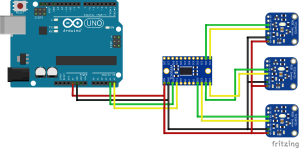
For a recent line-following robot competition at the RSSC, I was presented with a new challenge. The organizers made the path change colors along the way, forcing the robot to make decisions about which path to take when it came to an intersection. My typical line-following sensor of choice is an array of five generic infrared reflective sensors, which work great when there’s high-contrast between the lines and the field. However for this challenge, those sensors don’t have the color-spectrum range to get the job done. Adafruit manufactures a breakout circuit board based on the TCS34725 sensor which can detect the full RGB visible spectrum, has an on-board LED to reduce the effects of ambient light on the sensor output, and conveniently communicates via I2C. The basic line-following algorithm I used is to have 3 sensors in a line-array that are constantly scanning the ground and reporting back the color they see while the robot uses that data to try to keep itself centered on the right colored line. The TCS34725 chip has a fixed I2C address, so I also bought an I2C multiplexer breakout board which allows me to access all three sensors without network collisions.
-
-
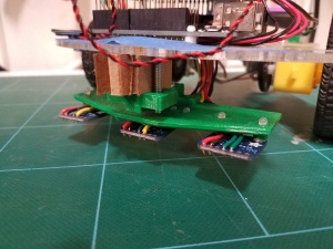
Robot Front View
-
-
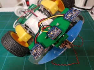
Robot Bottom View
-
-
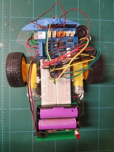
Robot Top View
-
-
Color Line Following Setup
The data from the color sensors comes in the form of an integer for each color Red, Green, and Blue and another integer for Clear light. My algorithm will need to take in that raw data and produce a prediction of what color the sensor is actually looking at all within the limitations of the Arduino. It would be somewhat difficult to train the algorithm and run it all on the Arduino, but the reality is: I don’t have to.
The whole process is actually two smaller processes, training and prediction. Training requires more processing power than prediction because it processes my entire collection of known data to work the prediction model down to the best fit for the data provided. Prediction on the other hand, is simple. It uses a simple math calculation called the sigmoid function which is easy to implement on the Arduino Uno and processes very quickly as well. I don’t need to train the algorithm on the Arduino. That can be done on the computer. Here’s an outline of the whole process:
Training
- Use the color sensors and an Arduino, connected to my computer to collect raw data.
- This is the supervised teaching method (i.e. a person is collecting the data and doing the work of picking what color it is up front.)
- The data will be output over the serial port and saved in a text file
- I need to know which color the sensor is trained on for each data set, so I’ll make one text file for each color
- To make the prediction robust, I’ll have to frequently change the position of the sensor and the lighting conditions
- The colored lines will always be near a white background, so I’ll need to collect data near those borders also
- Use Octave to import the data from the text files and use the fminunc function to quickly train the algorithm using gradient descent.
- When I import the data, I create an additional column that represents the known output from each set and assign a value; either 1 for match or 0 for not a match.
For example, if I’m training for finding Red, I’ll set all of the known outputs for the Red data set to 1 and all of the known outputs for the Blue, Green, Black, and White data to 0.
- Before training, I randomize the order of the data, mixing matches and non-matches, then set aside about 30% of the data points which I won’t use during training. After I’m done training, I’ll use the trained algorithm on this data to test if it’s working or not.
- The key part of the trained algorithm is the weights that I will use in the Arduino during real-time operation.
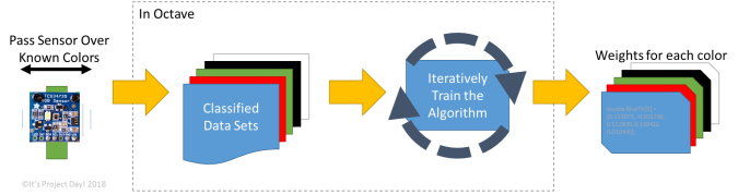
Training Process
Prediction
- During real-time operation, the Arduino will only use the prediction model.
- Unlike unsupervised learning algorithm, this prediction model will not “learn” any more than it already has learned at the time I program the Arduino
- The Arduino takes in the raw data, multiplies it by the weights, then passes the sum through the sigmoid function to decide if the color matches.
- I have to break the classification problem into a series of smaller problems. Instead of predicting “which color is it”, the Arduino will consider each color one-at-a-time as a yes/no question.
- The output isn’t guaranteed to be clear. For example, if the sensor is looking at a red/blue transition, it might produce a positive result for red and blue at the same time.
- I consider this possibility when writing the rest of my Arduino program.
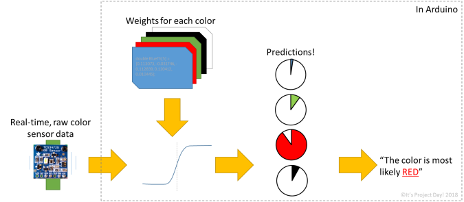
Prediction Process
If you’re new to machine learning and you want to dive deeper into using on your own, I recommend you check out Prof. Andrew Ng’s Machine Learning course on Coursera.
The algorithm worked out well for me. When I gathered data in my garage under LED light, the trained algorithm worked in that setting, probably very close to 99% success rate. On the day of the competition, the lights tended more toward the red end of the spectrum, so I gathered more data on the day and reran my training algorithm. After that, it worked fine. In general, gathering more data in more lighting conditions would help build robustness into the algorithm, but for a one-time-use project, it was good enough to get the job done. One major limitation I experienced was with the color sensor. It uses an accumulation time to gather data and that really hurt me on computation time. Every call to the sensor had a built-in 154ms delay, then multiply that by 3 sensors polled sequentially and the robot was very difficult to keep on-track. If I had more time, I might have tried to use something other than a delay, perhaps try to allow accumulation in parallel in the background and reduce the delay to 154ms total.
If you need a little help trying this out on your own, here is some sample code you can use to get started:
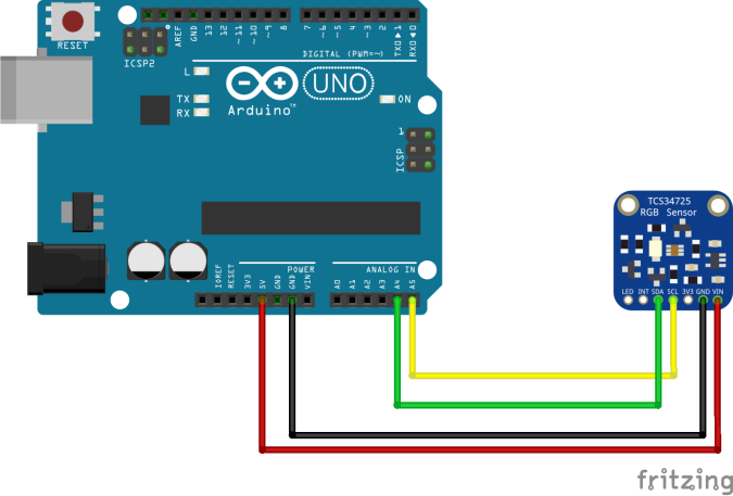
Arduino code for collecting the data to a text file:
-
-
Color Data Acquisition Setup
#include <Wire.h>
#include "Adafruit_TCS34725.h"
/* Initialize with specific int time and gain values */
Adafruit_TCS34725 tcs = Adafruit_TCS34725(TCS34725_INTEGRATIONTIME_154MS, TCS34725_GAIN_1X);
void RawColorPrint(int x[5]){
//debug code – color data for classifier
//Serial.print(x[0],DEC);Serial.print(“,”); // always = 1
Serial.print(x[1],DEC);Serial.print(“,”);
Serial.print(x[2],DEC);Serial.print(“,”);
Serial.print(x[3],DEC);Serial.print(“,”);
Serial.print(x[4],DEC);Serial.println(“”);
}
void setup() {
while(!Serial); //wait for Serial to start
delay(1000);
Wire.begin();
Serial.begin(115200);
Serial.println(“Starting…”);
delay(1000);
// Initialize the sensor
if (tcs.begin()) {
Serial.println(“Found sensor”);
} else {
Serial.println(“No TCS34725 found… check your connections”);
while (1);
}
}
void loop() {
//debug code – color data for classifier
uint16_t col0[5];
col0[0] = 1;
tcs.getRawData(&col0[1], &col0[2], &col0[3], &col0[4]);
RawColorPrint(col0);
}
Octave code for training the prediction algorithm:
sigmoid.m
function g = sigmoid(z)
g = zeros(size(z));
g = 1./(1.+exp(1).^(-z));
end
predict.m
function p = predict(theta, X)
m = size(X, 1); % Number of training examples
p = zeros(m, 1);
p = round(sigmoid(X*theta));
end
costFunction.m
function [J, grad] = costFunction(theta, X, y)
m = length(y); % number of training examples
J = 0;
grad = zeros(size(theta));
J = -((1/m)*sum(y.*log(sigmoid(X*theta))+(1.-y).*log(1.-sigmoid(X*theta))));
grad = (1/m)*sum((sigmoid(X*theta)-y).*X);
end
Main code:
%% Initialization
clear ; close all; clc
%% Load Data
Whidata = load(‘White.txt’);
Bladata = load(‘Black.txt’);
Bludata = load(‘Blue.txt’);
Reddata = load(‘Red.txt’);
Gredata = load(‘Green.txt’);
fprintf(‘Training for Red\n’)
%% Assign Match(1) to Red, and No Match(0) to all the rest
data = [Reddata ones(size(Reddata)(1),1)];
data = [data; Bladata zeros(size(Bladata)(1),1)];
data = [data; Bludata zeros(size(Bludata)(1),1)];
data = [data; Whidata zeros(size(Whidata)(1),1)];
data = [data; Gredata zeros(size(Gredata)(1),1)];
%% Randomize Order
data = data(randperm(size(data,1)),:);
%% Sequester 30% of the data for testing after training
datacutoff = int16(size(data)(1)*0.7);
X = data([1:datacutoff], [1:4]); y = data([1:datacutoff], 5);
Xtest = data([datacutoff + 1:size(data)(1)], [1:4]);
ytest = data([datacutoff + 1:size(data)(1)], 5);
%% Add constant term to X and Xtest
[m,n] = size(X);
X = [ones(size(X)(1), 1) X];
Xtest = [ones(size(Xtest)(1),1) Xtest];
%% Initialize weights
initial_theta = zeros(n + 1, 1);
%% Set options for fminunc
options = optimset(‘GradObj’, ‘on’, ‘MaxIter’, 10000);
%% Run fminunc to obtain the optimal weights
[theta, cost] = …
fminunc(@(t)(costFunction(t, X, y)), initial_theta, options);
%% Print weights to screen in Arduino-compatible format
fprintf(‘{%f, %f, %f, %f, %f} \n’, …
theta(1),theta(2),theta(3),theta(4),theta(5));
%% Use the optimal weights to predict the color of the checking data set
ycheck = predict(theta, Xtest);
fprintf(‘Train Accuracy: %f\n’, mean(double(ycheck == ytest)) * 100);
Arduino code for the prediction algorithm:
#include <Wire.h>
#include "Adafruit_TCS34725.h"
#define TCAADDR 0x70
/* Initialize with specific int time and gain values */
Adafruit_TCS34725 tcs0 = Adafruit_TCS34725(TCS34725_INTEGRATIONTIME_154MS, TCS34725_GAIN_1X);
Adafruit_TCS34725 tcs1 = Adafruit_TCS34725(TCS34725_INTEGRATIONTIME_154MS, TCS34725_GAIN_1X);
Adafruit_TCS34725 tcs2 = Adafruit_TCS34725(TCS34725_INTEGRATIONTIME_154MS, TCS34725_GAIN_1X);
/* Trained algorithm for 154ms delay and 1x gain */
double WhiteTh[5] = {-17.197105, -0.007517, 0.033887, -0.040166, 0.010233};
double BlackTh[5] = {13.863546, -0.011893, -0.022478, -0.013213, 0.005284};
double BlueTh[5] = {0.113073, -0.031746, -0.112839, 0.120412, 0.010445};
double RedTh[5] = {-0.051582, 0.077581, -0.036699, 0.042285, -0.027792};
double GreenTh[5] = {-12.740958, -0.187098, 0.227913, -0.174424, 0.033591};
void ClassifiedColorPrint(){
uint16_t col0[5], col1[5], col2[5];
col0[0] = 1;
col1[0] = 1;
col2[0] = 1;
tcaselect(0);
tcs0.getRawData(&col0[1], &col0[2], &col0[3], &col0[4]);
tcaselect(1);
tcs1.getRawData(&col1[1], &col1[2], &col1[3], &col1[4]);
tcaselect(2);
tcs2.getRawData(&col2[1], &col2[2], &col2[3], &col2[4]);
double B1Pred, B2Pred, WPred, RPred, GPred, MPred;
B1Pred = predict(col0,BlackTh);
B2Pred = predict(col0,BlueTh);
WPred = predict(col0,WhiteTh);
RPred = predict(col0,RedTh);
GPred = predict(col0,GreenTh);
//debug code – checking color classifier
Serial.println(” “);
Serial.println(“Sensor 0”);
Serial.print(“Black: “); Serial.println(B1Pred * 100.0);
Serial.print(“White: “); Serial.println(WPred * 100.0);
Serial.print(“Blue: “); Serial.println(B2Pred * 100.0);
Serial.print(“Red: “); Serial.println(RPred * 100.0);
Serial.print(“Green: “); Serial.println(GPred * 100.0);
B1Pred = predict(col1,BlackTh);
B2Pred = predict(col1,BlueTh);
WPred = predict(col1,WhiteTh);
RPred = predict(col1,RedTh);
GPred = predict(col1,GreenTh);
Serial.println(” “);
Serial.println(“Sensor 1”);
Serial.print(“Black: “); Serial.println(B1Pred * 100.0);
Serial.print(“White: “); Serial.println(WPred * 100.0);
Serial.print(“Blue: “); Serial.println(B2Pred * 100.0);
Serial.print(“Red: “); Serial.println(RPred * 100.0);
Serial.print(“Green: “); Serial.println(GPred * 100.0);
B1Pred = predict(col2,BlackTh);
B2Pred = predict(col2,BlueTh);
WPred = predict(col2,WhiteTh);
RPred = predict(col2,RedTh);
GPred = predict(col2,GreenTh);
Serial.println(” “);
Serial.println(“Sensor 2”);
Serial.print(“Black: “); Serial.println(B1Pred * 100.0);
Serial.print(“White: “); Serial.println(WPred * 100.0);
Serial.print(“Blue: “); Serial.println(B2Pred * 100.0);
Serial.print(“Red: “); Serial.println(RPred * 100.0);
Serial.print(“Green: “); Serial.println(GPred * 100.0);
}
void tcaselect(uint8_t i) {
if (i > 7) return;
Wire.beginTransmission(TCAADDR);
Wire.write(1 << i);
Wire.endTransmission();
}
double sigmoid(double z) {
return (double)1.0/((double)1.0 + exp(-z));
}
double predict(int x[5], double theta[5]) {
double answer = 0;
answer = ((double)x[0]*theta[0] + (double)x[1]*theta[1] + (double)x[2]*theta[2] + (double)x[3]*theta[3] + (double)x[4]*theta[4]);
answer = sigmoid(answer);
return answer;
}
void setup() {
while(!Serial); //wait for Serial to start
delay(1000);
Wire.begin();
Serial.begin(115200);
Serial.println(“Starting…”);
delay(1000);
// Initialize the sensors
tcaselect(0);
if (tcs0.begin()) {
Serial.println(“Found sensor”);
} else {
Serial.println(“No TCS34725 found on channel 0… check your connections”);
while (1);
}
tcaselect(1);
if (tcs1.begin()) {
Serial.println(“Found sensor”);
} else {
Serial.println(“No TCS34725 found on channel 1… check your connections”);
while (1);
}
tcaselect(2);
if (tcs2.begin()) {
Serial.println(“Found sensor”);
} else {
Serial.println(“No TCS34725 found on channel 2… check your connections”);
while (1);
}
}
void loop() {
//Print Classifications
ClassifiedColorPrint();
delay(1000);
}
For my code and these examples, I used the TCS34725 library from Adafruit and leaned heavily on their examples for the TCS34725 and TCA9548A.
FTC disclosure: this article contains affiliate links
If you liked this project, check out some of my others:
Instant Parade!
The ThrAxis – Our Scratch-Built CNC Mill
Fume Extractor
Did you like It’s Project Day? You can subscribe to email notifications by clicking ‘Follow’ in the side bar on the right, or leave a comment below.